Sol — a sunny little virtual machine
During this weekend, together with a few evenings earlier this week, I created a rather simple virtual machine dubbed “Sol”, after the Swedish word for “sun”. I’ve read a lot about VM design and I’m into stuff like OS design, programming languages and other seeminlgy obscure and nerdy stuff surrounding the concept of a computer as a generic tool.
A virtual machine (VM) is a software implementation of a machine (i.e. a computer) that executes programs like a physical machine. — Wikipedia
Sol is a process virtual machine that runs inside an operating system process. However, inside Sol there are multiple tasks (just like most operating systems have processes) and so for a program running in Sol it does not matter what the world looks like on the outside. We could even make Sol boot directly from hardware, but that would just be crazytown. Trust me. I’ve been down that road before.
The purpose of Sol is learning. As we are defining our world, we have an extremely high degree of freedom. One major component of a virtual machine is the provided instruction set. An instruction is the simplest type of operation that a program can perform, and so the set of instructions provided by the virtual machine to programs running in it need to be universal and efficient.
Design overview
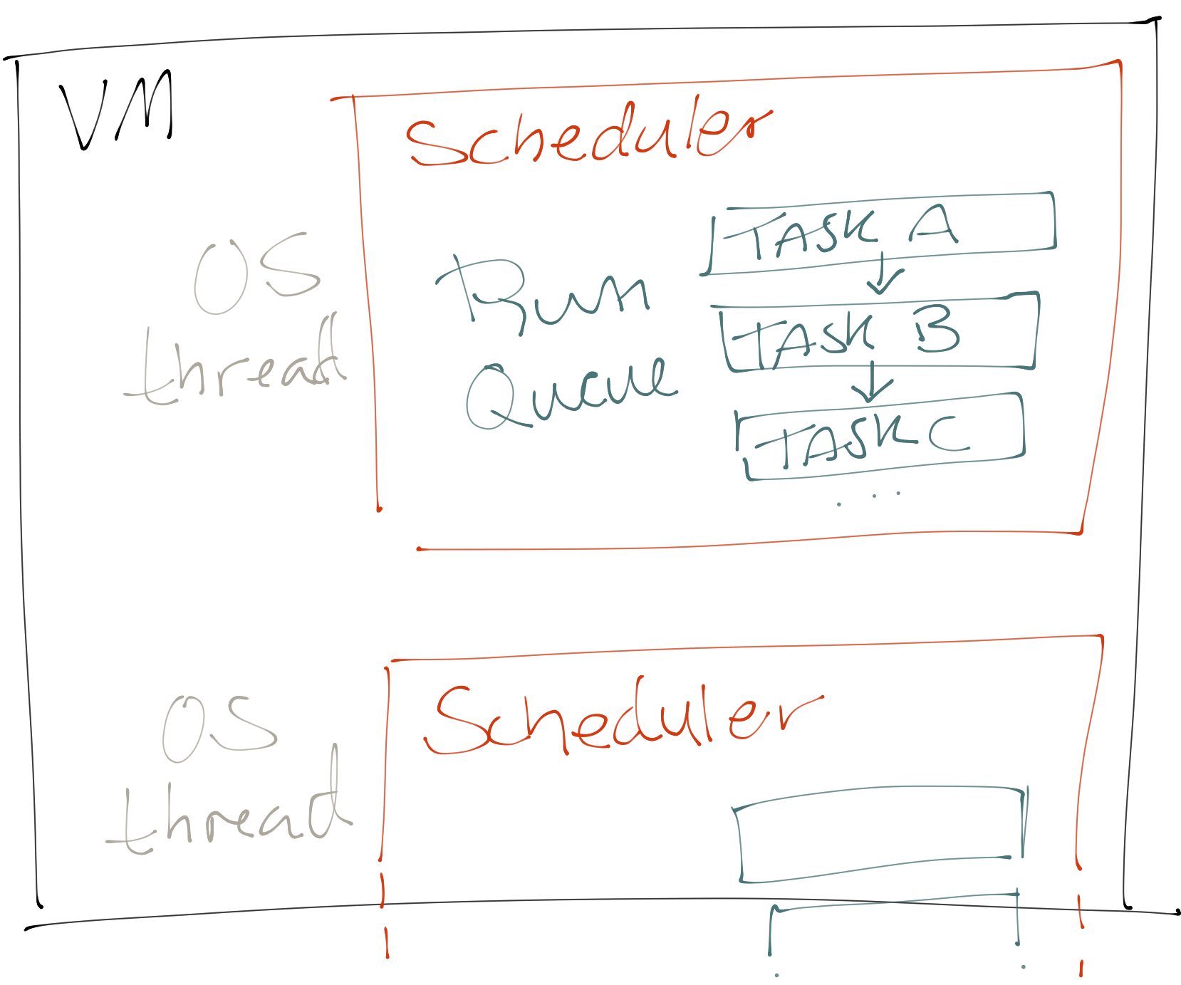
In the Sol VM there are one or more schedulers, each running on one CPU core (not yet implemented at the time of writing this).
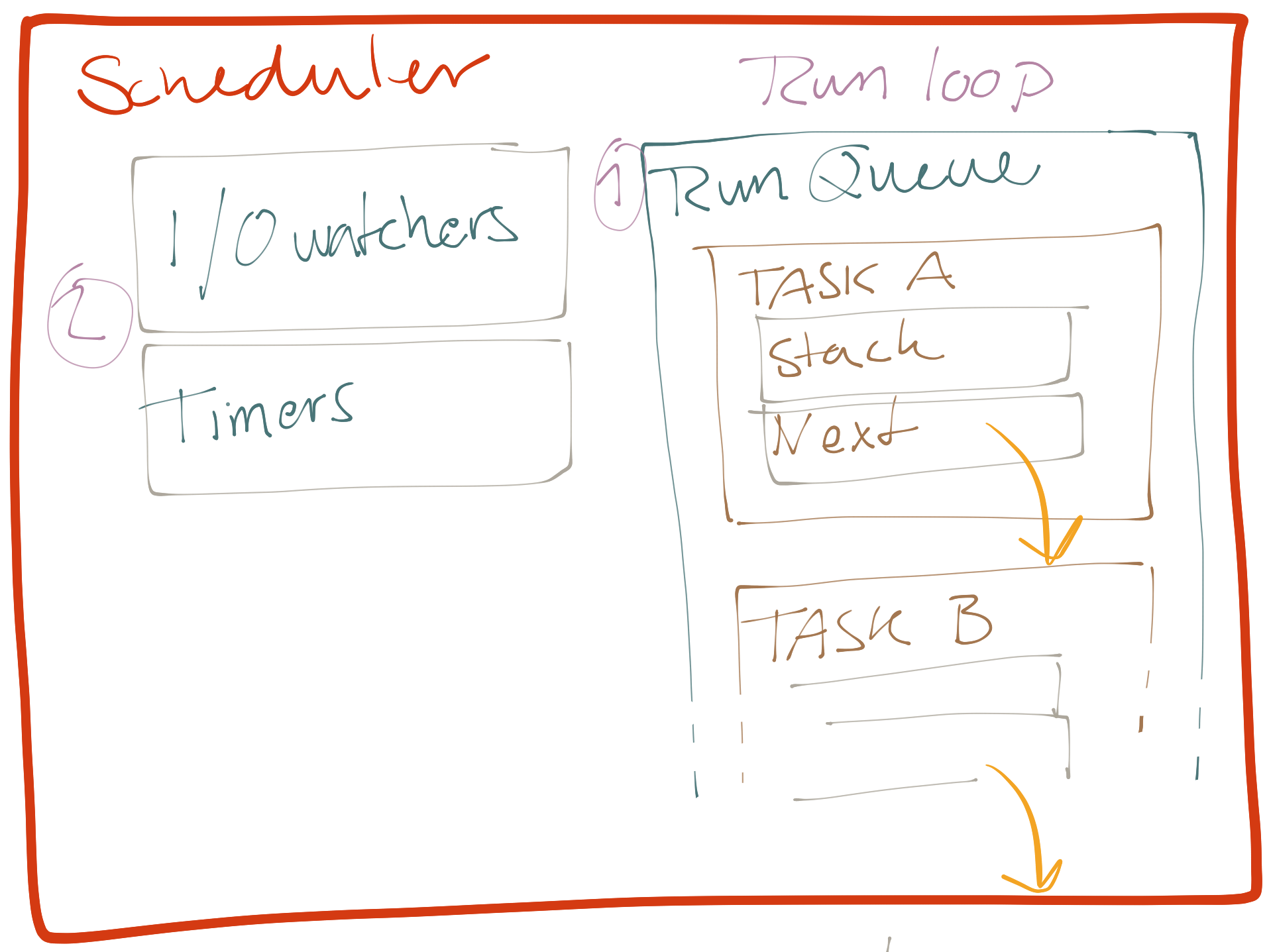
Each scheduler maintains a list of tasks to be run. This list is called the run queue. A scheduler also maintains I/O watchers, timers, handles OS interrupts, etc. The scheduler does most of the work in Sol as it not only does all those fancy things I just described, but it also executes program code.
The run queue is a list of tasks ordered in the way they are scheduled.
-
The scheduler takes the first task in the list from the run queue
-
executes the task (more on what that means later).
-
If the task ended with an “end” or “error” status, the task is removed from the run queue…
-
…otherwise places the task at the end of the list.
-
If there are any I/O watchers or timers, check timers for expiry and possibly call the host OS kernel to check on pending “asynchronous” I/O events.
- If an event has happened, like a timer expired or fired, the correlating task is added to the run queue so that the task can read the event it is waiting for.
-
The scheduler repeats this process (e.g. starting from point 1.) as long as there are any tasks in the run queue.
Let’s have a look at a task:
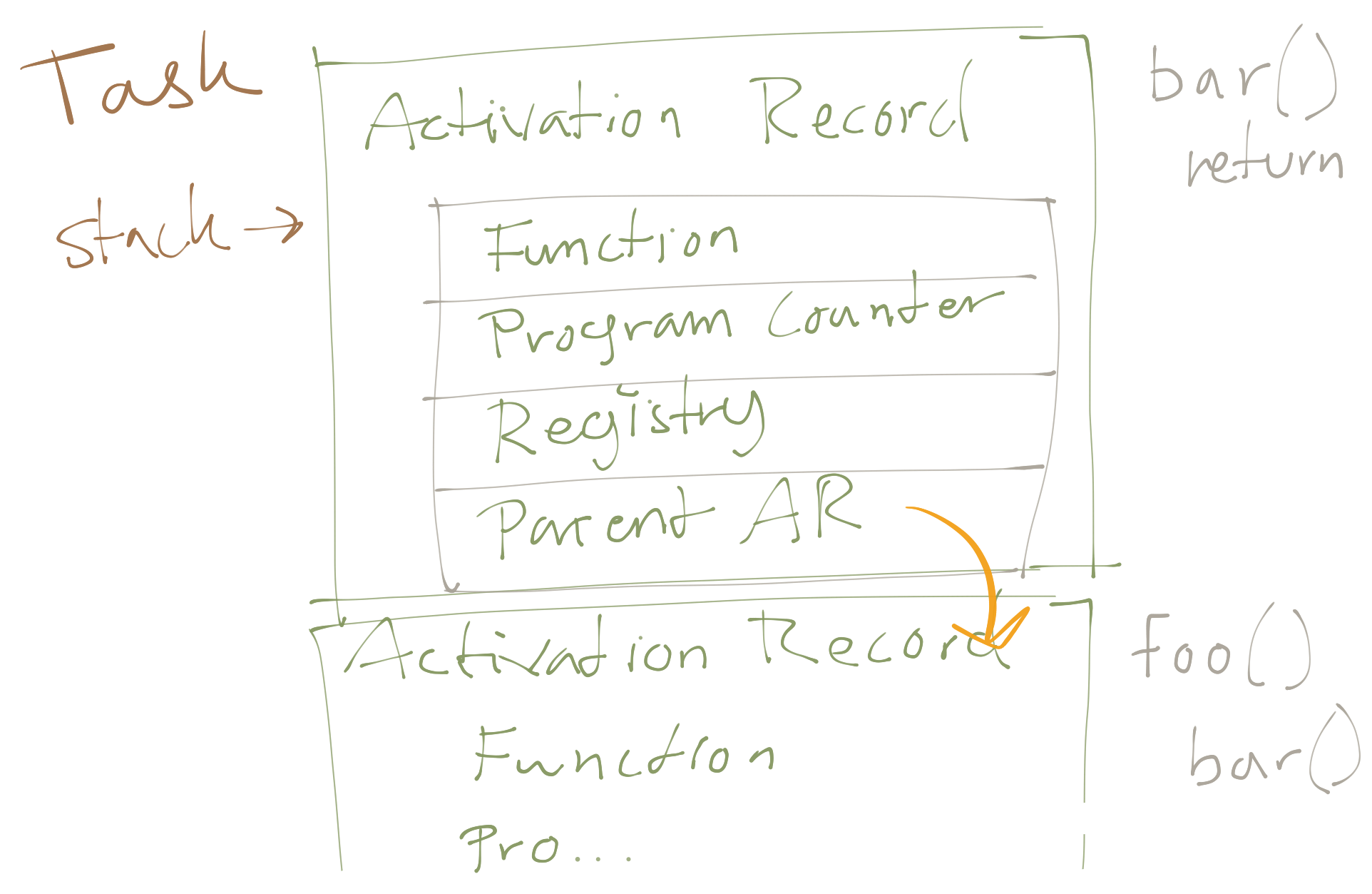
As we can see, a task is mostly an abstraction and contains only one significant component: Activation records. These comprise a task’s call stack and each activation record corresponds to one (active) function call. An activation record contains a reference to the function prototype (more on this in just a second) it’s executing, a program counter (usually called PC) which is a cursor for the currently executing program instruction and finally a registry for values.
A function prototype is the constants and the instruction of a function, but without a context (or “function closure”) with local variables etc. A function prototype is kind of like a building without any people or furniture. Albeit the name, it’s not really comparable to a blueprint as a function prototype is not copied or implemented, but is actually used as-is.
The program counter is simply a number that corresponds to an offset into the function prototype’s program (ordered list of instructions). As an activation record (we can think about this as a piece of running code) is executed, the program counter (PC) is incremented as each instruction is executed. Sometimes the PC is decremented, when a program jumps backwards (e.g. when performing a loop). The PC plays a central role in an instruction-based program (like your computer or phone’s hardware which is most likely incrementing a PC right now).
The registry is essentially a region of temporary memory that the executing program can use to store variable data. Imagine this simple function:
def foo(x, y):
  x = x * 5
  x = x * y
  return x
Here the program needs a way to store the value created by x * 5 that it can then pass to x * y which also needs to store its resulting value somewhere before using it with return. All local variables are stored in registers and thus access is very efficient. Something like this happens when executing the “foo” function (“R(x)” means “register x”):
argument 0 and 1 are already in R(0) and R(1)
load constant "5" into R(2)
multiply value-of R(0) with value-of R(2), put the result in R(0)
multiply value-of R(0) with value-of R(1), put the result in R(0)
return R(0)
Sol is a register-based virtual machine. Operands and results are read and stored from and to numbered registers, rather than “pushed” and “popped” to and from a stack (as with stack-based virtual machines). Register-based virtual machines avoid the push and pop operations usually surrounding other instructions, reducing code size, but in several cases also increases speed of execution (compared to stack-based virtual machines).
In the most excellent paper “The Implementation of Lua 5.0” Roberto, Luiz and Waldemar describes the (not really a) problem with code size and decoding overhead:
There are two problems usually associated with register-based machines: code size and decoding overhead. An instruction in a register machine needs to specify its operands, and so it is typically larger than a corresponding instruction in a stack machine. (For instance, the size of an instruction in Lua’s virtual machine is four bytes, while the size of an instruction in several typical stack machines, including the ones previously used by Lua, is one or two bytes.) On the other hand, register machines generate less opcodes than stack machines, so the total code size is not much larger.
Sol takes a lot of inspiration from Lua as well as Erlang.
Instructions and operations
An instruction consists of one or more components:
- An operation code (e.g. “subtract a from b”)
- 0-3 operands (e.g. “register a and register b, results in register c”)
As a virtual machine has the disadvantage of being …virtual, we must do whatever we can in terms of assuring good performance, so one of these instructions fit into one machine word. Most hardware today is able to deal with 32-bit long chunks of data very efficiently, so inspired by Lua 5 I chose a 32-bit representation for Sol’s instructions.
Each instruction and its operands is encoded in one of three layouts (Behold, awesome ASCII art!.)
OP ABC — Operation OP with operands A, B and C:
0         5 | 6          13 | 14           22 | 23            31   Bit
------------|---------------|-----------------|-----------------
     OP     |       A       |        B        |        C           Field
------------|---------------|-----------------------------------
     6              8                9                 9           Bits
  [0..63]        [0..255]         [0..511]          [0..511]       Range
Some operations only need two operands and can be made more efficient if one of those operands is large enough for common values. For this need we define an alternate layout of an instruction:
| OP ABx — Operation OP with operands A and Bs | Bu: |
0         5 | 6          13 | 14                              31   Bit
------------|---------------|-----------------------------------
     OP     |       A       |              Bs/Bu                   Field
------------|---------------|-----------------------------------
     6              8                        18                    Bits
  [0..63]        [0..255]             Bu: [0..262143]              Range
                                      Bu: [-131071..131072]
A third class of operations only use one operand which size has a correlation with efficiency, so we define a third alternate layout of an instruction where the three operands are effectively collapsed into one 26-bit integer value:
| OP Bxx — Operation OP with operand Bss | Buu: |
0         5 | 6                                               31   Bit
------------|---------------------------------------------------
     OP     |                     Bss/Buu                          Field
------------|---------------------------------------------------
     6                               26                            Bits
  [0..63]                   Buu: [0..67108863]                     Range
                            Bss: [-33554431..33554432]
A, B, C, Bu and Buu signify unsigned integers whilst Bs and Bss signify signed integers. As we can read above, there’s room for 64 operations and 256 registers (OP=6 bits, A=8 bits) with this configuration. More than we need :)
Changing and maintaining instructions (operations + operands) is simple in Sol. I’ve intentionally gone to great lengths in order to make playing around with the instuction set easy. The file instr.h contains a list of instructions:
/* Control flow */ \
_(YIELD,      ABC) /* suspend and reschedule */\
_(JUMP,       Bss) /* PC += Bss */\
_(CALL,       ABC) /* R(A), ... ,R(A+C-1) := R(A)(R(A+1), ... ,R(A+B)) */\
_(RETURN,     AB_) /* return R(A), ... ,R(A+B-1) */\
/* Data */ \
_(LOADK,      ABu) /* R(A) = K(Bu) */\
_(MOVE,       AB_) /* R(A) = R(B) */\
_(DBGREG,     ABC) /* special: Debug dump register values */\
/* Arithmetic */ \
_(ADD,        ABC) /* R(A) = RK(B) + RK(C) */\
_(SUB,        ABC) /* R(A) = RK(B) - RK(C) */\
_(MUL,        ABC) /* R(A) = RK(B) * RK(C) */\
...
Sol’s source code is setup in such a way that changing this list is all that is required, apart from the actual implementation of each instruction. Adding or renaming an instruction automatically makes convenience symbols and functions available. Say that we add a DING instruction which plays a little sound every time it’s executed:
_(MUL,        ABC) /* R(A) = RK(B) * RK(C) */\
_(DING,       Buu) /* A = sound number to play */\
...
There’s now a new operation identifier available called S_OP_DING as well as constructor function for encoding DING instructions:
SInstr SInstr_DING(uint32_t value);
Running a program now that includes a DING operation will cause an error in the VM: “unexpected operation”. We haven’t implemented the DING behavior yet! Operations are (at the time of writing this) implemented in sched_exec.h which is the core of the virtual machine as this is what reads and performs the instructions of a Sol program. It can be summed up like this:
void Execute(Instr* instructions) {
  Instr* pc = instructions;
  while (1) {
    switch (*++pc) {
    case S_OP_LOADK:
      // Read operands A and B from instruction *pc.
      // Put constant at B into register A.
      break;

    case S_OP_MOVE:
      // Read operands A and B from instruction *pc.
      // Put value of register B in register A.
      break;

    ...

    } // switch
  } // while
}
Pretty much a good old switch loop. When this C code is compiled with a modern compiler like Clang or GCC, it will be rather efficient as each of our virtual operations effectively corresponds to only a few machine instructions. This is where we need to add DING.
    ...
    case S_OP_DING:
      // Read operand Buu from instruction *pc.
      uint32_t sound_index = SInstrGetBuu(*pc);
      // Find note for sound_index and play it
      SoundNote* note = SoundGetNote(sound_index);
      SoundPlay(note);
      break;
    ...
Here the type Sound as well as SoundGet and SoundPlay represents some kind of sound playing function that you provide. Now we can write Sol programs that play music:
define melody 0
  entry:
  DING   0      # play note 0
  DING   1      # play note 1
  DING   1      # play note 1
  DING   2      # play note 2
  DING   0      # play note 0
  RETURN 0  0   # return
Pling, plong, plong, ding, pling!
Multitasking
No toy VM can be presented without shame unless it’s able to multitask; perform multiple things at once, or at least give the programmer the illusion of concurrency.
Sol has an operation called “yield” which is able to pause a task in any state and later have that task resume at the exact same state.
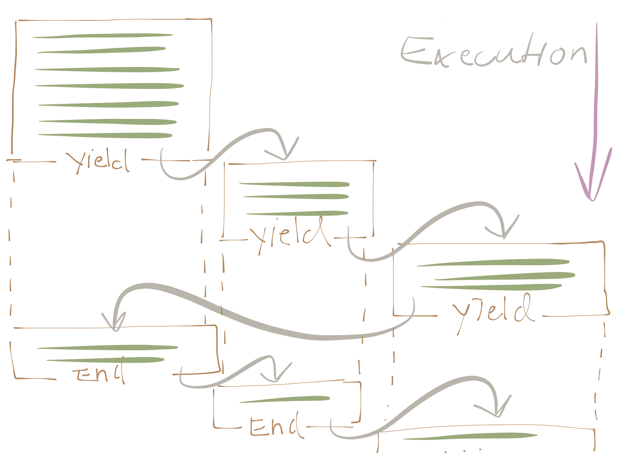
From the task’s perspective it never knew it was paused and resumed. This is a powerful primitive as we can implement many features on top of this. At the time of writing, Sol already has two different types of yield: Yielding for other tasks (so they can run or be scheduled from I/O etc events), and yielding for a timer to expire. At the end of this article there are a few example programs, all of them making use of yield.
Yield is used to implement cooperative multitasking where all tasks cooperate for the use of processing resources. When a task has performed a series of computations and relieves control to another task, one of three things has happened:
- The task initiated an external (“blocking”) operation, like reading from a file or waiting for a certain time to occur,
- the task completed and ended (it’s “main” function returned.),
- or the task faulted, caused an error.
Most systems that communicate with its environment and abroad, like a web server or a text editor, spend most of its time (CPU time relative to real time) waiting for the environment to respond; e.g. producing data on a network socket, writing contents to a file or returning a stepper motors position. These systems often benefit from cooperative multitasking, in particular coherent, specialized systems (unlike operating systems which are general by nature).
What Sol provides is essentially coroutines for concurrency. A nice feature with coroutines (aka “green threads” aka “user threads”) is their ability to run sequential code in a concurrent system. A task like this:
def read_file(name):
  f = open(name)
  data = read(f)
  close(f)
  return data
Involves three “blocking” calls to the environment which causes the task to yield:
openasks the operating system to open a file byname. The file might get opened sometime in the future. The scheduler takes a note that the task is waiting for this to happen, removes it from the run queue for the time being.- The OS tells the scheduler that “that file you wanted me to open, well here’s the file descriptor” and thus the scheduler places the task on the run queue again.
- The task receives the file descriptor representing the opened file
- The task again calls to the environment, this time asking to
readthe contents off. - Same thing as before, the scheduler tells the OS, takes a note, unschedules the task and continue with executing other tasks.
- The OS tells the scheulder “I’ve read that file you asked me to read, here’s the data” (in reality this is slightly more complicated, but the principles are the same)
- The scheduler queues the task, runs it.
- Same thing with the
closefunction.
For the programmer it’s easy to follow the flow of her program.
Comparing the above synchronous program to an asynchronous version:
def read_file(name, callback):
  open(name, def (error, f):
    if (error):
      callback(error)
    else:
      read(f, def (read_error, data):
        close(f, def (error):
          callback(error, data)
        )
      )
  )
  # returns here before the file has been opened
Clearly harder to follow. A task in Sol can spawn new tasks in order to perform several things at the same time, like writing a file while replying over the network.
def write_and_reply(destination_id, message):
  writer = write_file(destination_id + ".msg", message)
  send_message(destination_id, message)
  while (recv(writer) != TaskEnd) noop  # wait for write_file to end
However, as the Wikipedia section on cooperative multitasking mentions…
Because a cooperatively multitasked system relies on each process regularly giving up time to other processes on the system, one poorly designed program can consume all of the CPU time for itself or cause the whole system to hang.
This can happen when a program performs a very lengthy set of computations and can cause all kinds of problems, especially for other tasks relying on timers. As the Sol scheduler checks for timer expiration only between execution of tasks, a timer might effectively fire long after it was supposed to. Imagine controlling a toy quadrotor where one task needs to update one rotor’s angle each 50 milliseconds, and another task consumes a wholesome 200 milliseconds, then your quadrotor might just crash and burn.
To address this Sol employs an operation cost counter. Each task is given a predefined amount of “operation value” per execution iteration (when the scheduler runs a task’s program). When the operation cost counter reaches its limit, the task is simply forced to yield to other tasks. In the source code, look for S_VM_EXEC_LIMIT.
Some examples
The code below is expressed in a simplified assembly language that is almost 1:1 with the C API for defining these programs programatically, and so the assembly language itself should be considered irrelevant beyond explaining the instructions executed.
-
In the output, lines like these:
[vm] ______________ ...denote when the scheduler regains control after running a task and the task either returned or yielded. This is one “execution iteration”. When running multiple tasks, you will usually see tasks interleved in round-robin order between these “execution iteration” marker lines. -
In the output, lines starting with “…” are comments and/or simplifications and not part of the actual output.
-
In assembly comments,
R(x)means “Register x”,RK(x)means “Register x if x is less than k else Constant (x-k)” where k is a special value,K(x)means “Constant x”. -
In assembly comments,
PCsignifies the “program counter” which is sort of a cursor to the instructions of a program. It is incremented by one for each instruction executed. Some instructions will further modify this counter, like for instance theJUMPinstruction.
Example 1: while x > 0 yield …
While the variable x is greater than zero, decrement x by one and yield to the
scheduler, letting other tasks run. Eventually return.
def main():
  x = 5
  while (x > 0):
    x = x - 1
    yield
  return
Assembly:
define main 0
  CONST 5           # K(0) = 5
  CONST 0           # K(1) = 0
  CONST 1           # K(2) = 1
  entry:
  LOADK  0  0       # R(0) = K(0)
  LE     0  0  256  # (0 == RK(k+1) < RK(0)) ? continue else PC++
  JUMP   3          # PC += 3 to RETURN
  SUB    0  0  257  # R(0) = R(0) - RK(k+1)
  YIELD  0  0  0    # yield A=type=sched
  JUMP   -5         # PC -= 5 to LE
  RETURN 0  0       # return
Output when running in debug mode:
$ build/debug/bin/sol
Sol 0.1.0 x64
[vm] ______________ ______________ __________ _______ ____ ______________
[vm] Task           Function       PC         Op      Values
[vm] 0x7fdf28c03c00 0x7fdf28c000e0 0          LOADK   AB:    0,   0
[vm] 0x7fdf28c03c00 0x7fdf28c000e0 1          LE      ABC:   0,   0, 256
[vm] 0x7fdf28c03c00 0x7fdf28c000e0 3          SUB     ABC:   0,   0, 257
[vm] 0x7fdf28c03c00 0x7fdf28c000e0 4          YIELD   ABC:   0,   0,   0
[vm] ______________ ______________ __________ _______ ____ ______________
[vm] Task           Function       PC         Op      Values
[vm] 0x7fdf28c03c00 0x7fdf28c000e0 5          JUMP    Bss:       -5
[vm] 0x7fdf28c03c00 0x7fdf28c000e0 1          LE      ABC:   0,   0, 256
[vm] 0x7fdf28c03c00 0x7fdf28c000e0 3          SUB     ABC:   0,   0, 257
[vm] 0x7fdf28c03c00 0x7fdf28c000e0 4          YIELD   ABC:   0,   0,   0
[vm] ______________ ______________ __________ _______ ____ ______________
...three more execution iterations identical to the above block...
[vm] ______________ ______________ __________ _______ ____ ______________
[vm] Task           Function       PC         Op      Values
[vm] 0x7fdf28c03c00 0x7fdf28c000e0 5          JUMP    Bss:       -5
[vm] 0x7fdf28c03c00 0x7fdf28c000e0 1          LE      ABC:   0,   0, 256
[vm] 0x7fdf28c03c00 0x7fdf28c000e0 2          JUMP    Bss:        3
[vm] 0x7fdf28c03c00 0x7fdf28c000e0 6          RETURN  AB:    0,   0
Scheduler runloop exited.
Example 2: Function calls and timers
This program uses two functions. The entry point is the main function which simply
calls the kitten function with one argument ‘500’. The kitten function “sleeps” for
the number of milliseconds passed to it (as the first argument.) The kitten function
then returns the number “123” to the caller—the main function—which dumps register values and
finally returns, causing the task to exit and subsequently the scheduler and the VM too to exit.
Assembly:
define kitten 1     # Arguments: (R(0)=sleep_ms)
  CONST  123        # K(0) = 123
  entry:
  YIELD  1  0  0    # yield A=type=timer, RK(B)=R(0)=arg0
  LOADK  0  0       # R(0) = K(0) = 123
  RETURN 0  1       # return R(0)..R(0) = R(0) = 123

define main 0       # Arguments: ()
  CONST  @kitten    # K(0) = <func kitten>
  CONST  500        # K(1) = 500
  entry:
  LOADK  0  0       # R(0) = K(0) = the kitten function
  LOADK  1  1       # R(1) = K(1) = 500
  CALL   0  1  1    # R(0)..R(0) = R(0)(R(1)..R(1)) = a(R(1))
  DBGREG 0  1  0    # VM debug function that dumps register values
  RETURN 0  0       # return
Output when running in debug mode:
$ time build/debug/bin/sol
Sol 0.1.0 x64
[vm] ______________ ______________ __________ _______ ____ ______________
[vm] Task           Function       PC         Op      Values
[vm] 0x7f8c9bc03bf0 0x7f8c9bc03910 0          LOADK   AB:    0,   0
[vm] 0x7f8c9bc03bf0 0x7f8c9bc03910 1          LOADK   AB:    1,   1
[vm] 0x7f8c9bc03bf0 0x7f8c9bc03910 2          CALL    ABC:   0,   1,   1
[vm] 0x7f8c9bc03bf0 0x7f8c9bc000e0 1          YIELD   ABC:   1,   0,   0
D Timer scheduled to trigger after 500.000000 ms (sched.c:81)
# ...time passes and in this case the scheduler is idling...
D Timer triggered -- scheduling task (sched.c:57)
[vm] ______________ ______________ __________ _______ ____ ______________
[vm] Task           Function       PC         Op      Values
[vm] 0x7f8c9bc03bf0 0x7f8c9bc000e0 2          LOADK   AB:    0,   0
[vm] 0x7f8c9bc03bf0 0x7f8c9bc000e0 3          RETURN  AB:    0,   1
[vm] 0x7f8c9bc03bf0 0x7f8c9bc03910 3          DBGREG
D [vm] R(0) = 123.000000 (sched_exec.h:214)
D [vm] R(1) = 500.000000 (sched_exec.h:215)
D [vm] R(0) = 123.000000 (sched_exec.h:216)
[vm] 0x7f8c9bc03bf0 0x7f8c9bc03910 4          RETURN  AB:    0,   0
Scheduler runloop exited.

real  0m0.504s
user  0m0.001s
sys   0m0.001s
Example 3: Multitasking
Here we run three tasks, each running the program in Example 1:
$ build/debug/bin/sol
Sol 0.1.0 x64
[sched 0x7fc219403930] run queue:
  [task 0x7fc219403c00] -> [task 0x7fc219403cd0] -> [task 0x7fc219403da0]
[vm] ______________ ______________ __________ _______ ____ ______________
[vm] Task           Function       PC         Op      Values
[vm] 0x7fc219403c00 0x7fc2194000e0 0          LOADK   AB:    0,   0
[vm] 0x7fc219403c00 0x7fc2194000e0 1          LE      ABC:   0,   0, 256
[vm] 0x7fc219403c00 0x7fc2194000e0 3          SUB     ABC:   0,   0, 257
[vm] 0x7fc219403c00 0x7fc2194000e0 4          YIELD   ABC:   0,   0,   0
[vm] ______________ ______________ __________ _______ ____ ______________
[vm] Task           Function       PC         Op      Values
[vm] 0x7fc219403cd0 0x7fc2194000e0 0          LOADK   AB:    0,   0
[vm] 0x7fc219403cd0 0x7fc2194000e0 1          LE      ABC:   0,   0, 256
[vm] 0x7fc219403cd0 0x7fc2194000e0 3          SUB     ABC:   0,   0, 257
[vm] 0x7fc219403cd0 0x7fc2194000e0 4          YIELD   ABC:   0,   0,   0
[vm] ______________ ______________ __________ _______ ____ ______________
[vm] Task           Function       PC         Op      Values
[vm] 0x7fc219403da0 0x7fc2194000e0 0          LOADK   AB:    0,   0
[vm] 0x7fc219403da0 0x7fc2194000e0 1          LE      ABC:   0,   0, 256
[vm] 0x7fc219403da0 0x7fc2194000e0 3          SUB     ABC:   0,   0, 257
[vm] 0x7fc219403da0 0x7fc2194000e0 4          YIELD   ABC:   0,   0,   0
[vm] ______________ ______________ __________ _______ ____ ______________
[vm] Task           Function       PC         Op      Values
[vm] 0x7fc219403c00 0x7fc2194000e0 5          JUMP    Bss:       -5
[vm] 0x7fc219403c00 0x7fc2194000e0 1          LE      ABC:   0,   0, 256
[vm] 0x7fc219403c00 0x7fc2194000e0 3          SUB     ABC:   0,   0, 257
[vm] 0x7fc219403c00 0x7fc2194000e0 4          YIELD   ABC:   0,   0,   0
[vm] ______________ ______________ __________ _______ ____ ______________
# The above block of instruction is repeated three times in interleved
# round-robin order for each task. Then:
[vm] ______________ ______________ __________ _______ ____ ______________
[vm] Task           Function       PC         Op      Values
[vm] 0x7fc219403c00 0x7fc2194000e0 5          JUMP    Bss:       -5
[vm] 0x7fc219403c00 0x7fc2194000e0 1          LE      ABC:   0,   0, 256
[vm] 0x7fc219403c00 0x7fc2194000e0 2          JUMP    Bss:        3
[vm] 0x7fc219403c00 0x7fc2194000e0 6          RETURN  AB:    0,   0
[vm] ______________ ______________ __________ _______ ____ ______________
[vm] Task           Function       PC         Op      Values
[vm] 0x7fc219403cd0 0x7fc2194000e0 5          JUMP    Bss:       -5
[vm] 0x7fc219403cd0 0x7fc2194000e0 1          LE      ABC:   0,   0, 256
[vm] 0x7fc219403cd0 0x7fc2194000e0 2          JUMP    Bss:        3
[vm] 0x7fc219403cd0 0x7fc2194000e0 6          RETURN  AB:    0,   0
[vm] ______________ ______________ __________ _______ ____ ______________
[vm] Task           Function       PC         Op      Values
[vm] 0x7fc219403da0 0x7fc2194000e0 5          JUMP    Bss:       -5
[vm] 0x7fc219403da0 0x7fc2194000e0 1          LE      ABC:   0,   0, 256
[vm] 0x7fc219403da0 0x7fc2194000e0 2          JUMP    Bss:        3
[vm] 0x7fc219403da0 0x7fc2194000e0 6          RETURN  AB:    0,   0
Scheduler runloop exited.
Source code
Released free under a very permissive MIT-style license at https://github.com/rsms/sol.